Table of contents
- In this note, $\{x_i\}^b_a$ denotes set $\{x_a, x_{a+1}, \ldots, x_b\}$
- TODO: add Jordan Form
Algebraic Structures
Operation
- Definition: an (binary, closed) operation $\ast$ on a set $S$ is a mapping of $S\times S\to S$
- Commutative: $x\ast y=y\ast x,\;\forall x,y\in S$
- Associative: $(x\ast y)\ast z=x\ast (y\ast z),\;\forall x,y,z\in S$
Group
- Definition: a group is a pair $(\mathcal{S},\ast)$ with following axioms
- $\ast$ is associative on $\mathcal{S}$
- (Identity element) $\exists e\in \mathcal{S}\text{ s.t. }x\ast e=e\ast x=x,\;\forall x\in \mathcal{S}$
- (Inverse element) $\forall x\in \mathcal{S}, \exists x’ \in \mathcal{S}\text{ s.t. }x\ast x’=x’\ast x=e$
- Abelian: a group is called abelian group if $\ast$ is also commutative
Ring
- Definition: a ring is a triplet $(\mathcal{R},+,\ast)$ consisting of a set of
scalars$\mathcal{R}$ and two operators + and $\ast$ with following axioms- $(\mathcal{R},+)$ is an abelian group with identity denoted $0$
- $\forall a,b,c \in \mathcal{R}\text{ s.t. }a\ast(b\ast c) = (a\ast b)\ast c$
- $\exists 1\in\mathcal{R}, \forall a\in\mathcal{R}\text{ s.t. }a\cdot 1=a$
- $\ast$ is distributive over $+$
Field
- Definition: a field $(\mathcal{F},+,\ast)$ is a ring where $(\mathcal{F}\backslash\{0\},\ast)$ is also an abelian group.
Difference from ring to field is that $\ast$ need to be commutative and have a multiplicative inverse
Vector Space
- Definition: a vector space (aka. linear space) is a triplet $(\mathcal{U},\oplus,\cdot)$ defined over a field $(\mathcal{F},+,\ast)$ with following axioms, where set $\mathcal{U}$ is called
vectors, operator $\oplus$ is calledvector additionand mapping $\cdot$ is calledscalar multiplication:- (Null vector) $(\mathcal{U},+)$ is an abelian group with identity element $\emptyset$
- Scalar multiplication is a mapping of $\mathcal{F}\times\mathcal{U}\to\mathcal{U}$
- $\alpha\cdot(x\oplus y) = \alpha\cdot x \oplus \alpha\cdot y,\;\forall x,y\in\mathcal{U};\alpha\in\mathcal{F}$
- $(\alpha+\beta)\cdot x = \alpha\cdot x\oplus\beta\cdot x,\;\forall x\in\mathcal{U};\alpha,\beta\in\mathcal{F}$
- $(\alpha\ast\beta)\cdot x=\alpha\cdot(\beta\cdot x),\;\forall x\in\mathcal{U};\alpha,\beta\in\mathcal{F}$
- $1_\mathcal{F}\cdot x=x$
Usually we don’t distinguish vector addition $\oplus$ and addition of scalar $+$. Juxtaposition is also commonly used for both scalar multiplication $\cdot$ and multiplication of scalars $\ast$
- Subspace: a subspace $\mathcal{V}$ of a linear space $\mathcal{U}$ over field $\mathcal{F}$ is a subset of $\mathcal{U}$ which is itself a linear space over $\mathcal{F}$ under same vector addition and scalar multiplication.
Basis & Coordinate
- Linear Independence: Let $\mathcal{V}$ be a vector space over $\mathcal{F}$ and let $X=\{x_i\}^n_1\subset \mathcal{V}$
- X is linearly dependent if $\exists \alpha_1,\ldots,\alpha_n\in\mathcal{F}$ not all 0 s.t. $\sum^n_{i=1} \alpha_i x_i=0$.
- X is linearly independent if $\sum^n_{i=1} \alpha_i x_i=0 \Rightarrow \alpha_1=\alpha_2=\ldots=\alpha_n=0$
- Span: Given a set of vectors $V$, the set of linear combinations of vectors in $V$ is called the span of it, denoted $\mathrm{span}\{V\}$
- Basis: A set of linearly independent vectors in a linear space $\mathcal{V}$ is a basis if every vector in $\mathcal{V}$ can be expressed as a unique linear combination of these vectors. (see below “Coordinate”)
- Basis Expansion: Let $(X,\mathcal{F})$ be a vector space of dimension n. If $\{v_i\}^k_1,\;1\leqslant k< n$ is linearly independent, then $\exists \{v_i\}^n_{k+1}$ such that $\{v_i\}_1^n$ is a basis.
- Reciprocal Basis: Given basis $\{v_i\}^n_1$, a set ${r_i}^1_n$ that satifies $\langle r_i,v_j \rangle=\delta_i(j)$ is a reciprocal basis. It can be generated by Gram-Schmidt Process and $\forall x\in\mathcal{X}, x=\sum^n_{i=1}\langle r_i,x\rangle v_i$.
- Dimension: Cardinality of the basis is called the dimension of that vector space, which is equal to the maximum number of linearly independent vectors in the space. Denoted as $dim(\mathcal{V})$.
- In an $n$-dimensional vector space, any set of $n$ linearly independent vectors is a basis.
- Coordinate: For a vector $x$ in vector space $\mathcal{V}$, given a basis $\{e_1, \ldots, e_n\}$ we can write $x$ as $x=\sum^n_{i=1}\beta_i e_i=E\beta$ where $E=\begin{bmatrix}e_1&e_2&\ldots&e_n\end{bmatrix}$ and $\beta=\begin{bmatrix}\beta_1&\beta_2&\ldots&\beta_n\end{bmatrix}^\top$. Here $\beta$ is called the representation (or coordinate) of $x$ given the basis $E$.
Norm & Inner product
- Inner Product: an operator on two vectors that produces a scalar result (i.e. $\langle\cdot,\cdot\rangle:\mathcal{V}\to\mathbb{R}\;or\;\mathbb{C}$) with following axioms:
- (Symmetry) $\langle x,y \rangle=\overline{\langle y,x\rangle},\;\forall x,y\in\mathcal{V}$
- (Bilinearity) $\langle \alpha x+\beta y,z\rangle=\alpha\langle x,z\rangle+\beta\langle y,z\rangle,\;\forall x,y,z\in\mathcal{V};\alpha,\beta\in\mathbb{C}$
- (Pos. definiteness) $\langle x,x\rangle\geqslant 0,\;\forall x\in\mathcal{V}$ and $\langle x,x\rangle=0\Rightarrow x=0_\mathcal{V}$
- Inner Product Space: A linear space with a defined inner product
- Orthogonality:
- Perpedicularity of vectors ($x\perp y$): $\langle x,y\rangle=0$
- Perpedicularity of a vector to a set ($y\perp\mathcal{S},\mathcal{S}\subset\mathcal{V}$): $y\perp x,\;\forall x\in\mathcal{S}$
- Orthogonal Set: set $\mathcal{S}\subset(\mathcal{U},\langle\cdot,\cdot\rangle)$ is orthogonal $\Leftrightarrow x\perp y,\;\forall x,y\in\mathcal{S},x\neq y$
- Orthonormal Set: set $\mathcal{S}$ is orthonormal iff $\mathcal{S}$ is orthogonal and $\Vert x\Vert=1,\;\forall x\in\mathcal{S}$
- Orthogonality of sets ($\mathcal{X}\perp\mathcal{Y}$): $\langle x,y\rangle=0,\;\forall x\in\mathcal{X};y\in\mathcal{Y}$
- Orthogonal Complement: Let $(\mathcal{V},\langle\cdot,\cdot\rangle)$ be an inner product space and let $\mathcal{U}\subset\mathcal{V}$ be a subspace of $\mathcal{V}$, the orthogonal complement of $\mathcal{U}$ is $\mathcal{U}^\perp=\left\{v\in\mathcal{V}\middle|\langle v,u\rangle=0,\;\forall u\in\mathcal{U}\right\}$.
- $\mathcal{U}^\perp\subset\mathcal{V}$ is a subspace
- $\mathcal{V}=\mathcal{U}\overset{\perp}{\oplus}\mathcal{U}^\perp$ ($\oplus$: direct sum, $\overset{\perp}{\oplus}$: orthogonal sum)
- Norm: A norm on a linear space $\mathcal{V}$ is mapping $\Vert\cdot\Vert:\;\mathcal{V}\to\mathbb{R}$ such that:
- (Positive definiteness) $\Vert x\Vert\geqslant 0\;\forall x\in \mathcal{V}$ and $\Vert x\Vert =0\Rightarrow x=0_\mathcal{V}$
- (Homogeneous) $\Vert \alpha x\Vert=|\alpha|\cdot\Vert x\Vert,\;\forall x\in\mathcal{V},\alpha\in\mathbb{R}$
- (Triangle inequality) $\Vert x+y\Vert\leqslant\Vert x\Vert+\Vert y\Vert$
- Distance: Norm can be used to measure distance between two vectors. Meanwhile, distance from a vector to a (sub)space is defined as $d(x,\mathcal{S})=\inf_{y\in\mathcal{S}} d(x,y)=\inf_{y\in\mathcal{S}} \Vert x-y\Vert$
- Projection Point: $x^* =\arg\min_{y\in\mathcal{S}}\Vert x-y\Vert$ is the projection point of $x$ on linear space $\mathcal{S}$.
- Projection Theorem: $\exists !x^* \in\mathcal{S}$ s.t. $\Vert x-x^* \Vert=d(x,\mathcal{S})$ and we have $(x-x^*) \perp\mathcal{S}$
- Orthogonal Projection: $P(x)=x^*:\mathcal{X}\to\mathcal{M}$ is called the orthogonal projection of $\mathcal{X}$ onto $\mathcal{M}$
- Normed Space: A linear space with a defined norm $\Vert\cdot\Vert$, denoted $(\mathcal{V},\mathcal{F},\Vert\cdot\Vert)$
A inner product space is always a normed space because we can define $\Vert x\Vert=\sqrt{\langle x,x\rangle}$
- Common $\mathbb{R}^n$ Norms:
- Euclidean norm (2-norm): $\Vert x\Vert_2=\left(\sum^n_{i=1}|x_i|^2\right)^{1/2}=\left\langle x,x\right\rangle^{1/2}=\left(x^\top x\right)^{1/2}$
- $l_p$ norm (p-norm): $\Vert x\Vert_p=\left(\sum^n_{i=1}|x_i|^p\right)^{1/p}$
- $l_1$ norm: $\Vert x\Vert_1=\sum^n_{i=1}|x_i|$
- $l_\infty$ norm: $\Vert x\Vert_\infty=\max_{i}\{x_i\}$
- Common matrix norms:
Matrix norms are also called operator norms, can measure how much a linear operator “magnifies” what it operates on.
- A general form induced from $\mathbb{R}^n$ norm: $$\Vert A\Vert=\sup_{x\neq 0}\frac{\Vert Ax\Vert}{\Vert x\Vert}=\sup_{\Vert x\Vert=1}\Vert Ax\Vert$$
- $\Vert A\Vert_1=\max_j\left(\sum^n_{i=1}|a_{ij}|\right)$
- $\Vert A\Vert_2=\left[ \max_{\Vert x\Vert=1}\left\{(Ax)^* (Ax)\right\}\right]^{1/2}=\left[ \lambda_{max}(A^ *A)\right]^{1/2}$ ($\lambda_{max}$: largest eigenvalue)
- $\Vert A\Vert_\infty=\max_i\left(\sum^n_{j=1}|a_{ij}|\right)$
- (Frobenius Norm) $\Vert A\Vert_F=\left[ \sum^m_{i=1}\sum^n_{j=1}\left|a_{ij}\right|^2\right]^{1/2}=\left[ tr(A^*A)\right]^{1/2}$
- Useful inequations:
- Cauchy-Schwarz: $|\langle x,y\rangle|\leqslant\left\langle x,x\right\rangle^{1/2}\cdot\left\langle y,y\right\rangle^{1/2}$
- Triangle (aka. $\Delta$): $\Vert x+y\Vert\leqslant\Vert x\Vert+\Vert y\Vert$
Lemma: $\Vert x-y\Vert \geqslant \left| \Vert x\Vert-\Vert y\Vert \right|$
- Pythagorean: $x\perp y \Leftrightarrow \Vert x+y\Vert=\Vert x\Vert+\Vert y\Vert$
Gramian
- Gram-Schmidt Process: A method to find orthogonal basis $\{v_i\}^n_1$ given an ordinary basis $\{y_i\}^n_1$. It’s done by perform $v_k=y_k-\sum^{k-1}_{j=1}\frac{\langle y_k,v_j\rangle}{\langle v_j,v_j \rangle}\cdot v_j$ iteratively from 1 to $n$. To get an orthonormal basis, just normalize these vectors.
- Gram Matrix: The Gram matrix generated from vectors $\{y_i\}_ 1^k$ is denoted $G(y_ 1,y_ 2,\ldots,y_ k)$. Its element $G_{ij}=\langle y_i,y_j\rangle$
- Gram Determinant: $g(y_1,y_2,\ldots,y_n)=\det G$
- Normal Equations: Given subspace $\mathcal{M}$ and its basis $\{y_i\}^n_1$, the projection point of $\forall x\in\mathcal{M}$ can be represented by $$x^*=\alpha y=\begin{bmatrix}\alpha_1&\alpha_2&\ldots&\alpha_n\end{bmatrix}\begin{bmatrix}y_1\\y_2\\ \vdots \\y_n\end{bmatrix},\;\beta=\begin{bmatrix}\langle x,y_1\rangle\\ \langle x,y_2\rangle\\ \vdots\\ \langle x,y_n\rangle\end{bmatrix} where\;G^\top\alpha=\beta$$
For least-squares problem $Ax=b$, consider $\mathcal{M}$ to be the column space of $A$, then $G=A^\top A,\;\beta=A^\top b,\;G^\top\alpha=\beta\Rightarrow\alpha=(A^\top A)^{-1}A^\top b$. Similarly for weighted least-squares problem ($\Vert x\Vert=x^\top Mx$), let $G=A^\top MA, \beta=A^\top Mb$, we can get $\alpha=(A^\top MA)^{-1}A^\top Mb$
Linear Algebra
Linear Operator
Definition: a linear operator $\mathcal{A}$ (aka. linear transformation, linear mapping) is a function $f: V\to U$ that operate on a linear space $(\mathcal{V},\mathcal{F})$ to produce elements in another linear space $(\mathcal{U},\mathcal{F})$ and obey $$\mathcal{A}(\alpha_1 x_1+\alpha_2 x_2) = \alpha_1\mathcal{A}(x_1) + \alpha_2\mathcal{A}(x_2),\;\forall x_1,x_2\in V;\alpha_1, \alpha_2\in\mathcal{F}$$
Range (Space): $\mathcal{R}(\mathcal{A})=\left\{u\in U\middle|\mathcal{A}(v)=u,\;\forall v\in V\right\}$
Null Space (aka. kernel): $\mathcal{N}(\mathcal{A})=\left\{v\in V\middle|\mathcal{A}(v)=\emptyset_U\right\}$
$\mathcal{A}$-invariant subspace: Given vector space $(\mathcal{V},\mathcal{F})$ and linear operator $\mathcal{A}:\mathcal{V}\rightarrow \mathcal{V}$, $\mathcal{W}\subseteq\mathcal{V}$ is $A$-invariant if $\forall x\in\mathcal{W}$, $\mathcal{A}x\in\mathcal{W}$.
- Both $\mathcal{R}(\mathcal{A})$ and $\mathcal{N}(\mathcal{A})$ are $\mathcal{A}$-invariant
Matrix Representation: Given bases for both $V$ and $U$ (respectively $\{v_i\}^n_1$ and $\{u_j\}^m_1$), matrix representation $A$ satisfies $\mathcal{A}(v_i)=\sum^m_{j=0}A_{ji}u_j$ so that $\beta=A\alpha$ where $\alpha$ and $\beta$ is the representation of a vector under $\{v_i\}$ and $\{u_j\}$ respectively.
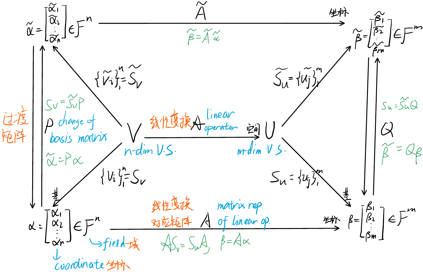
- $P$ and $Q$ are change of basis matrices, $A=Q^{-1}\tilde{A}P,\;\tilde{A}=QAP^{-1}$
- The i-th column of $A$ is the coordinates of $\mathcal{A}(v_i)$ represented by the basis $\{u_j\}$, similarly i-th column of $\tilde{A}$ is $\mathcal{A}(\tilde{v}_i)$ represented in $\{\tilde{u}_j\}$
- The i-th column of $P$ is the coordinates of $v_i$ represented by the basis $\{\tilde{v}\}$, similarly i-th column of $Q$ is $u_j$ represented in $\{\tilde{u}\}$
Matrix Similarity ($A\sim B$): Two (square) matrix representations ($A,B$) of the same linear operator are called similar (or conjugate) and they satisfies $\exists P$ s.t. $B=PAP^{-1}$.
From now on we don’t distinguish between linear operator $\mathcal{A}$ and its matrix representation where choice of basis doesn’t matter.
Rank: $rank(A)=\rho(A)\equiv dim(\mathcal{R}(A))$
- Sylvester’s Inequality: $\rho(A)+\rho(B)-n\leqslant \rho(AB)\leqslant \min\{\rho(A), \rho(B)\}$
- Singularity: $\rho(A)< n$
Nullity: $null(A)=\nu(A)\equiv dim(\mathcal{N}(A))$
- $\rho(A)+\nu(A)=n$ ($n$ is the dimensionality of domain space)
Adjoint: The adjoint of the linear map $\mathcal{A}: \mathcal{V}\to\mathcal{W}$ is the linear map $\mathcal{A}^*: \mathcal{W}\to\mathcal{V}$ such that $\langle y,\mathcal{A}(x)\rangle_\mathcal{W}=\langle \mathcal{A}^ *(y),x\rangle_\mathcal{V}$
For its matrix representation, adjoint of $A$ is $A^ *$, which is $A^\top$ for real numbers.
Properties of $\mathcal{A}^ *$ is similar to matrix $A^ *$- $\mathcal{U}=\mathcal{R}(A)\overset{\perp}{\oplus}\mathcal{N}(A^ *),\;\mathcal{V}=\mathcal{R}(A^ *)\overset{\perp}{\oplus}\mathcal{N}(A)$
- $\mathcal{N}(A^* )=\mathcal{N}(AA^* )\subseteq\mathcal{U},\;\mathcal{R}(A)=\mathcal{R}(AA^*)\subseteq\mathcal{U}$
Self-adjoint: $\mathcal{A}$ is self-adjoint iff $\mathcal{A}^*=\mathcal{A}$.
- For self-adjoint $\mathcal{A}$, if $\mathcal{V}=\mathbb{C}^{n\times n}$ then $A$ is hermitian; if $\mathcal{V}=\mathbb{R}^{n\times n}$ then $A$ is symmetric.
- Self-adjoint matrices have real eigenvalues and orthogonal eigenvectors
- Skew symmetric: $A^*=-A$
For quadratic form $x^\top Ax=x^\top(\frac{A+A^\top}{2}+\frac{A-A^\top}{2})x$, since $A-A^\top$ is skew symmetric, scalar $x^\top (A-A^\top) x=-x^\top (A-A^\top)x$, so the skew-symmetric part is zero. Therefore for quadratic form $x^\top Ax$ we can always assume $A$ is symmetric.
Definiteness: (for symmetric matrix $P$)
- Positive definite ($P\succ 0$): $\forall x\in\mathbb{R}^n\neq 0,\; x^\top Px>0 \Leftrightarrow$ all eigenvalues of $P$ are positive.
- Semi-positive definite ($P\succcurlyeq 0$): $x^\top Px\geqslant 0 \Leftrightarrow$ all eigenvalues of $P$ are non-negative.
- Negative definite ($P\prec 0$): $x^\top Px < 0 \Leftrightarrow$ all eigenvalues of $P$ are negative.
Orthogonal Matrix: $Q$ is orthogonal iff $Q^\top Q=I$, iff columns of $Q$ are orthonormal.
- If $A\in\mathbb{R}^{n\times b}$ is symmetric, then $\exists$ orthogonal $Q$ s.t. $Q^\top AQ=\Lambda=\mathrm{diag}\{\lambda_1,\ldots,\lambda_n\}$ (see Eigen-decomposition section below)
Orthogonal Projection: Given linear space $\mathcal{X}$ and subspace $\mathcal{M}$, $P(x)=x^*:\mathcal{X}\to\mathcal{M}$ ($x^ *$ is the projection point) is called orthogonal projection. If $\{v_i\}$ is a orthonormal basis of $\mathcal{M}$, then $P(x)=\sum_i \langle x,v_i\rangle v_i$
Eigenvalue and Canonical Forms
- Eigenvalue and Eigenvector: Given mapping $\mathcal{A}:\mathcal{V}\rightarrow\mathcal{V}$, if $\exists \lambda\in\mathcal{F}, v\neq \emptyset_{\mathcal{V}}\in\mathcal{V}$ s.t. $\mathcal{A}(v) = \lambda v$, then $\lambda$ is the eigenvalue, $v$ is the eigenvector (aka. spectrum).
- If eigenvalues are all distinct, then the associated eigenvectors form a basis.
- Eigenspace: $\mathcal{N}_\lambda = \mathcal{N}(\mathcal{A}-\lambda \mathcal{I})$.
- $q=dim(\mathcal{N}_\lambda)$ is called the geometric multiplicity (几何重度)
- $\mathcal{N}_\lambda$ is an $\mathcal{A}$-invariant subspace.
- Characteristic Polynomial: $\phi(s)\equiv\mathcal{det}(A-s I)$ is a polynomial of degree $n$ in $s$
- Its solutions are the eigenvalues of $A$.
- The multiplicity $m_i$ of root term $(s-\lambda_i)$ here is called algebraic multiplicity (代数重度) of $\lambda_i$.
- Cayley-Hamilton Theorem: $\phi(A)=\mathbf{0}$
Proof needs the eigendecomposition or Jordan decomposition descibed below
- Minimal Polynomial: $\psi(s)$ is the minimal polynomial of $A$ iff $\psi(s)$ is the polynomial of least degree for which $\psi(A)=0$ and $\psi$ is monic (coefficient of highest order term is 1)
- The multiplicity $\eta_i$ of root term $(s-\lambda_i)$ here is called the index of $\lambda_i$
- Eigendecomposition (aka. Spectral Decomposition) is directly derived from the definition of eigenvalues: $$A=Q\Lambda Q^{-1}, \Lambda=\mathrm{diag}\left\{\lambda_1,\lambda_2,\ldots,\lambda_n\right\}$$
where $Q$ is a square matrix whose $i$-th column is the eigenvector $q_i$ corresponding to eigenvalue $\lambda_i$.
- Feasibility: $A$ can be diagonalized (using eigendecomposition) iff. $q_i=m_i$ for all $\lambda_i$.
- If $A$ has $n$ distinct eigenvalues, then $A$ can be diagonalized.
- Generalized eigenvector: A vector $v$ is a generalized eigenvector of rank $k$ associated with eigenvalue $\lambda$ iff $v\in\mathcal{N}\left((A-\lambda I)^k\right)$ but $v\notin\mathcal{N}\left((A-\lambda I)^{k-1}\right)$
- If $v$ is a generalized eigenvector of rank $k$, $(A-\lambda I)v$ is a generalized eigenvector of rank $k-1$. This creates a chain of generalized eigenvectors (called Jordan Chain) from rank $k$ to $1$, and they are linearly independent.
- $\eta$ (index, 幂零指数) of $\lambda$ is the smallest integer s.t. $dim\left(\mathcal{N}\left((A-\lambda I)^\eta\right)\right)$
- The space spanned by the chain of generalized eigenvectors from rank $\eta$ is called the generalized eigenspace (with dimension $\eta$).
- Different generalized eigenspaces associated with the same and with different eigenvalues are orthogonal.
- Jordan Decomposition: Similar to eigendecomposition, but works for all square matrices. $A=PJP^{-1}$ where $J=\mathrm{diag}\{J_1,J_2,\ldots,J_p\}$ is the Jordan Form of A consisting of Jordan Blocks.
- Jordan Block: $J_i=\begin{bmatrix} \lambda & 1 &&& \\&\lambda&1&&\\&&\lambda&\ddots&\\&&&\ddots&1\\&&&&\lambda\end{bmatrix}$
- Each Jordan block corresponds to a generalized eigenspace
- $q_i$ = the count of Jordan blocks associated with $\lambda_i$
- $m_i$ = the count of $\lambda_i$ on diagonal of $J$
- $\eta_i$ = the dimension of the largest Jordan block associated with $\lambda_i$
$\Lambda$ in eigendecomposition, $J$ in Jordan Form and $\Sigma$ in SVD (see below) are three kinds of Canonical Forms of a matrix $A$
- Function of matrics: Let $f(\cdot)$ be an analytic function and $\lambda_i$ be an eigenvalue of $A$. If $p(\cdot)$ is a polynomial that satisfies $p(\lambda_i)=f(\lambda_i)$ and $\frac{\mathrm{d}^k}{\mathrm{d}s^k} p(\lambda_i)=\frac{\mathrm{d}^k}{\mathrm{d}s^k} f(\lambda_i)$ for $k=1,\ldots,\eta_i-1$, then $f(A)\equiv p(A)$.
- This extends the functions applicable to matrics from polynomials (trivial) to any analytical functions
- By Cayley-Hamilton, we can always choose $p$ to be order $n-1$
- Sylvester’s Formula: $f(A)=\sum^k_{i=1}f(\lambda_i)A_i$ ($f$ being analytic)
SVD and Linear Equations
SVD Decomposition is useful in various fields and teached by a lot of courses, its complete version is formulated as $$A=U\Sigma V^*, \Sigma=\begin{bmatrix}\mathbf{\sigma}&\mathbf{0}\\ \mathbf{0}&\mathbf{0}\end{bmatrix}, \mathbf{\sigma}=\mathrm{diag}\left\{\sqrt{\lambda_1},\sqrt{\lambda_2},\ldots,\sqrt{\lambda_r}\right\},V=\begin{bmatrix}V_1&V_2\end{bmatrix},U=\begin{bmatrix}U_1&U_2\end{bmatrix}$$ where
- $r=\rho(A)$ is the rank of matrix $A$
- $\sigma_i$ are called sigular values, $\lambda_i$ are eigenvalues of $A^* A$
- Columns of $V_1$ span $\mathcal{R}(A^ *A)=\mathcal{R}(A^ *)$, columns of $V_2$ span $\mathcal{N}(A^ *A)=\mathcal{N}(A)$
- Columns of $U_1=AV_1\sigma^{-1}$ span $\mathcal{R}(A)$, columns of $U_2$ span $\mathcal{N}(A^*)$
SVD can be derived by doing eigenvalue decomposition on $A^* A$
With SVD introduced, we can efficiently solve general linear equation $Ax=b$ as $x=x_r+x_n$ where $x_r\in\mathcal{R}(A^\top)$ and $x_n\in\mathcal{N}(A)$.
| $Ax=b$ | tall $A$ ($m>n$) | fat $A$ ($m< n$) | |
|---|---|---|---|
| Overdetermined, Least Squares, use Normal Equations | Underdetermined, Quadratic Programming, use Lagrange Multiplies | ||
| I.$b\in\mathcal{R}(A)$ | |||
| 1.$\mathcal{N}(A)={0}$ | $x$ exist & is unique | $x=(A^\top A)^{-1}A^\top b=A^+b$ | $x=A^\top(AA^\top)^{-1}b=A^+b$ |
| 2.$\mathcal{N}(A)\neq{0}$ | $x$ exist & not unique | $x_r=(A^\top A)^{-1}A^\top b=A^+b$ | $x_r=A^\top(AA^\top)^{-1}b=A^+b$ |
| II.$b\notin\mathcal{R}(A)$ | |||
| 1.$\mathcal{N}(A)={0}$ | $x$ not exists, $x_r$ exist & is unique | $x_r=(A^\top A)^{-1}A^\top b=A^+b$ | $x_r=A^\top(AA^\top)^{-1}b=A^+b$ |
| 2.$\mathcal{N}(A)\neq{0}$ | $x$ not exists, $x_r$ not exist | $(A^\top A)^{-1}$ invertible | $(AA^\top)^{-1}$ invertible |
- $A^+=(A^\top A)^{-1}A^\top$ is left pseudo-inverse, $A^+=A^\top (AA^\top)^{-1}$ is right pseudo-inverse.
- $A^+$ can be unified by the name Moore-Penrose Inverse and calculated using SVD by $A^+=V\Sigma^+ U^\top$ where $\Sigma^+$ take inverse of non-zeros.
Miscellaneous
Selected theorems and lemmas useful in Linear Algebra. For more matrix properties see my post about Matrix Algebra
- Matrix Square Root: $N^\top N=P$, then $N$ is the square root of $P$
Square root is not unique. Cholesky decomposition is often used as square root.
- Schur Complement: Given matrices $A_{n\times n}, B_{n\times m}, C_{m\times m}$, the matrix $M=\begin{bmatrix}A&B\\ B^\top&C\end{bmatrix}$ is symmetric. Then the following are equivalent (TFAE)
- $M\succ 0$
- $A\succ 0$ and $C-B^\top A^{-1}B\succ 0$ (LHS called Schur complement of $A$ in $M$)
- $C\succ 0$ and $A-B C^{-1}B^\top\succ 0$ (LHS called Schur complement of $C$ in $M$)
- Matrix Inverse Lemma: $(A+BCD)^{-1}=A^{-1}-A^{-1}B\left(C^{-1}+DA^{-1}B\right)^{-1}DA$
- Properties of $A^\top A$
- $A^\top A \succeq 0$ and $A^\top A \succ 0 \Leftrightarrow A$ has full rank.
- $A^\top A$ and $AA^\top$ have same non-zero eigenvalues, but different eigenvectors.
- If $v$ is eigenvector of $A^\top A$ about $\lambda$, then $Av$ is eigenvector of $AA^\top$ about $\lambda$.
- If $v$ is eigenvector of $AA^\top$ about $\lambda$, then $A^\top v$ is eigenvector of $A^\top A$ about $\lambda$.
- $tr(A^\top A)=tr(AA^\top)=\sum_i\sum_j\left|A_{ij}\right|^2$
- $det(A)=\prod_i\lambda_i, tr(A)=\sum_i\lambda_i$
Real Analysis
Set theory
$\text{~}S$ stands for complement of set $S$ in following contents. These concepts are discussed under normed space $(\mathcal{X}, \Vert\cdot\Vert)$
- Open Ball: Let $x_0\in\mathcal{X}$ and let $a\in\mathbb{R}, a>0$, then the open ball of radius $a$ about $x_0$ is $B_a(x_0)=\left\{x\in\mathcal{X}\middle| \Vert x-x_0\Vert < a\right\}$
- Given subset $S\subset \mathcal{X}$, $d(x,S)=0\Leftrightarrow \forall\epsilon >0, B_\epsilon(x)\cap S\neq\emptyset$
- Given subset $S\subset \mathcal{X}$, $d(x,S)>0\Leftrightarrow \exists\epsilon >0, B_\epsilon(x)\cap S=\emptyset$
- Interior Point: Given subset $S\subset\mathcal{X}$, $x\in S$ is an interior point of $S$ iff $\exists\epsilon >0, B_\epsilon(x)\subset S$
- Interior: $\mathring{S}=\{x\in \mathcal{X}|x\text{ is an interior point of }S\}=\{x\in\mathcal{X}|d(x,\text{~}S)>0\}$
- Open Set: $S$ is open if $\mathring{S}=S$
- Closure Point: Given subset $S\subset\mathcal{X}$, $x\in S$ is a closure point of $S$ iff $\forall\epsilon >0, B_\epsilon(x)\cap S\neq\emptyset$.
- Closure: $\bar{S}=\{x\in\mathcal{X}|x\text{ is a closure point of }S\}=\{x\in\mathcal{X}|d(x,S)=0\}$
Note that $\partial\mathcal{X}=\emptyset$
- Closure: $\bar{S}=\{x\in\mathcal{X}|x\text{ is a closure point of }S\}=\{x\in\mathcal{X}|d(x,S)=0\}$
- Closed Set: $S$ is closed if $\bar{S}=S$
$S$ is open $\Leftrightarrow$ $\text{~}S$ is closed, $S$ is closed $\Leftrightarrow$ $\text{~}S$ is open. Set being both open and closed is called clopen(e.g. the whole set $\mathcal{X}$), empty set is clopen by convention.
- Set Boundary: $\partial S=\bar{S}\cap\overline{\text{~}S}=\bar{S}\backslash\mathring{S}$
Sequences
- Sequence($\{x_n\}$): a set of vectors indexed by the counting numbers
- Subsequence: Let $1\leqslant n_1< n_2<\ldots$ be an infinite set of increasing integers, then $\{x_{n_i}\}$ is a subsequence of $\{x_n\}$
- Convergence($\{x_n\}\to x\in\mathcal{X}$): $\forall \epsilon>0,\exists N(\epsilon)<\infty\text{ s.t. }\forall n\geqslant N, \Vert x_n-x\Vert <\epsilon$
- If $x_n \to x$ and $x_n \to y$, then $x=y$
- If $x_n \to x_0$ and $\{x_{n_i}\}$ is a subsequence of $\{x_n\}$, then $\{x_{n_i}\} \to x_0$
- Cauchy Convergence (necessary condition for convergence): $\{x_n\}$ is cauchy if $\forall \epsilon>0,\exists N(\epsilon)<\infty$ s.t. $\forall n,m\geqslant N, \Vert x_n-x_m\Vert <\epsilon$
- If $\mathcal{X}$ is finite dimensional, $\{x_n\}$ is cauchy $\Rightarrow$ $\{x_n\}$ has a limit in $\mathcal{X}$
- Limit Point: Given subset $S\subset\mathcal{X}$, $x$ is a limit point of $S$ if $\exists \{x_n\}$ s.t. $\forall n\geqslant 1, x_n\in S$ and $x_n\to x$
- $x$ is a limit point of $S$ iff $x\in\bar{S}$
- $S$ is closed iff $S$ contains its limit points
- Complete Space: a normed space is complete if every Cauchy sequence has a limit. A complete normed space $(\mathcal{X}, \Vert\cdot\Vert)$ is called a Banach space.
- $S\subset \mathcal{X}$ is complete if every Cauchy sequence with elements from $S$ has a limit in $S$
- $S\subset \mathcal{X}$ is complete $\Rightarrow S$ is closed
- $\mathcal{X}$ is complete and $S\subset\mathcal{X} \Rightarrow S$ is complete
- All finite dimensional subspaces of $X$ are complete
- Completion of Normed Space: $\mathcal{Y}=\bar{\mathcal{X}}=\mathcal{X}+\{$all limit points of Cauchy sequences in $\mathcal{X}\}$
E.g. $C[a,b]$ contains continuous functions over $[a,b]$. $(C[a,b], \Vert\cdot\Vert_1)$ is not complete, $(C[a,b], \Vert\cdot\Vert_\infty)$ is complete. Completion of $(C[a,b], \Vert\cdot\Vert_1)$ requires Lebesque integration.
- Contraction Mapping: Let $S\subset\mathcal{X}$ be a subset and $T:S\to S$ is a contraction mapping if $\exists 0\leqslant c\leqslant 1$ such that, $\forall x,y \in S, \Vert T(x)-T(y)\Vert\leqslant c\Vert x-y\Vert$
- Fixed Point: $x^* \in\mathcal{X}$ is a fixed point of $T$ if $T(x^ *)=x^ *$
- Contraction Mapping Theorem (不动点定理): If $T:S\to S$ is a contraction mapping in a complete subset $S$, then $\exists! x^ *\in\mathcal{X}\text{ s.t. }T(x^ *)=x^ *$. Moreover, $\forall x_0\in S$, the sequence $x_{k+1}=T(x_k),k\geqslant 0$ is Cauchy and converges to $x^ *$.
E.g. Newton Method: $x_{k+1}=x_k-\epsilon\left[\frac{\partial h}{\partial x}(x_k)\right]^{-1}\left(h(x_k)-y\right)$
Continuity and Compactness
- Continuous: Let $(\mathcal{X},\Vert\cdot\Vert_\mathcal{X})$ and $(\mathcal{Y},\Vert\cdot\Vert_\mathcal{Y})$ be two normed spaces. A function $f:\mathcal{X}\to\mathcal{Y}$ is continuous at $x_0\in\mathcal{X}$ if $\forall\epsilon >0,\exists \delta(\epsilon,x_0)>0\text{ s.t. }\Vert x-x_0\Vert_\mathcal{X}<\delta \Rightarrow\Vert f(x)-f(x_0)\Vert_\mathcal{Y} <\epsilon$
- $f$ is continuous on $S\subset\mathcal{X}$ if $f$ is continuous at $\forall x_0\in S$
- If $f$ in continuous at $x_0$ and $\{x_n\}$ is a sequence s.t. $x_n\to x_0$, then the sequence $\{f(x_n)\}$ in $\mathcal{Y}$ converges to $f(x_0)$
- If $f$ is discontinuous at $x_0$, then $\exists \{x_n\}\in\mathcal{X}$ s.t. $x_n\to x_0$ but $f(x_n)\nrightarrow f(x_0)$
- Compact: $S\subset\mathcal{X}$ is (sequentially) compact if every sequence in $S$ has a convergent subsequence with limit in $S$
- Bounded: $S\subset\mathcal{S}$ is bounded if $\exists r<\infty$ such that $S\subset B_r(0)$
- $S$ is compact $\Rightarrow$ $S$ is closed and bounded
- Bolzano-Weierstrass Theorem: In a finite-dimensional normed space, $C$ is closed and bounded $\Leftrightarrow$ for $C$ is compact
- Weierstrass Theorem: If $C\subset\mathcal{X}$ is a compact subset and $f:C\to\mathbb{R}$ is continuous at each point of $C$, then $f$ achieves its extreme values, i.e. $\exists \bar{x}\in C\text{ s.t. }f(\bar{x})=\sup_{x\in C} f(x)$ and $\exists \underline{x}\in C\text{ s.t. }f(\underline{x})=\inf_{x\in C} f(x)$
- $f:C\to\mathbb{R}$ continuous and $C$ compact $\Rightarrow$ $\sup_{x\in C}f(x)<\infty$
There is a very nice interactive text book for linear algebra FYI.