Table of contents
Probability Space
- Notation: $(\Omega,\mathcal{F},\mathbb{P})$
- $\Omega$: Sample space
- $\mathcal{F}$: Event space. Required to be σ-algebra. We often use Borel σ-algebra for continuous $\Omega$).
- Axioms for σ-algebra
- $\mathcal{F}$ is non-empty
- $A\in\mathcal{F} \Rightarrow A^C\in\mathcal{F}$ (closed under complement)
- $A_i \in\mathcal{F} \Rightarrow \bigcup^\infty_{k=1} A_k \in \mathcal{F}$ (closed under countable union)
- For continuous case considering interval $\Omega=[a,b]$, $\mathcal{F}_0$ is the set of all subintervals of $\Omega$. Then its Borel σ-algebra is the smallest σ-algebra that contains $\mathcal{F}_0$. Here the $\mathcal{F}_0$ is a semialgebra. We can find a containing σ-algebra for every semialgebra.
- Axioms for semialgebra
- $\emptyset, \Omega \in \mathcal{F}$
- $A_i \in\mathcal{F} \Rightarrow \bigcap^n_{k=1} A_k \in \mathcal{F}$ (closed under finite intersections)
- $\forall B \in\mathcal{F}, B^C=\bigcup^n_{k=1} A_k$ where $A_i \in \mathcal{F}$
- Axioms for σ-algebra
- $\mathbb{P}$: Probability measure.
- Axioms for probability measure
- $\mathbb{P}(\Omega) = 1$
- $\forall A\in\mathcal{F}, \mathbb{P}(A) \geqslant 0$
- $A_i, A_j \in\mathcal{F}$ are pairwise disjoint, then $\mathbb{P}(\bigcup^\infty_{k=1}A_k)=\sum^\infty_{k=1}\mathbb{P}(A_k)$
- Axioms for probability measure
- Product Space: Probability spaces can be combined using Cartesian product.
- Independence: $\mathbb{P}(A_{k_1}\cap A_{k_2}\cap …\cap A_{k_l})=\prod_{i=1}^l \mathbb{P}(A_i),\;\forall \{k_i\}_1^l\subset\{ 1..n\}$
- Conditional probability: $\mathbb{P}\left(A_i \middle| A_j\right)=\mathbb{P}(A_i\cap A_j)/\mathbb{P}(A_j)$
- Total probability: $\mathbb{P}(B)=\sum_{i=1}^n \mathbb{P}(B\cap A_i)=\sum_{i=1}^n \mathbb{P}\left(B\middle| A_i\right)\mathbb{P}(A_i)$, where $\{A_1,\cdots,A_n\}$ are disjoint and partition of $\Omega$.
- Bayes’ Rule: $$\mathbb{P}(A_j|B)=\frac{\mathbb{P}(B|A_j)\mathbb{P}(A_j)}{\sum^n_{i=1} \mathbb{P}(B|A_i)\mathbb{P}(A_i)}$$
- Priori: $\mathbb{P}(B|A_j)$
- Posteriori: $\mathbb{P}(A_j|B)$
Random Variables
Note: The equations are written in continuous case by default, one can get the equation for discrete case by changing integration into summation and changing differential into difference.
- Random Variable $\mathcal{X}$ is a mapping $\mathcal{X}: (\Omega,\mathcal{F},\mathbb{P})\to(\Omega_ \mathcal{X},\mathcal{F}_ \mathcal{X},\mathbb{P}_ \mathcal{X})$
- Continuous & Discrete & Mixed Random Variable:
- Can be defined upon whether $\Omega_\mathcal{X}$ is continuous
- Can be defined upon whether we can find continuous density function $f_\mathcal{X}$
- $\mathcal{F}_\mathcal{X}$ for continuous $\mathcal{X}$ is a Borel σ-field
- All three kinds of random variables can be expressed by CDF or “extended” PDF with Dirac function and Lebesgue integration.
- Scalar Random Variable: $\mathcal{X}: \Omega\to\mathbb{F}$
- Formal definition: $\mathcal{X}: (\Omega,\mathcal{F},\mathbb{P})\to(\Omega_ \mathcal{X}\subset\mathbb{F},\mathcal{F}_ \mathcal{X}\subset\left\{\omega\middle| \omega\subset\Omega_ \mathcal{X}\right\},\mathbb{P}_ \mathcal{X}:\mathcal{F}_ \mathcal{X}\to[0,1])$
- Cumulative Distribution Function (CDF): $F_ \mathcal{X}(x)=\mathbb{P}_\mathcal{X}(\mathcal{X}(\omega)\leqslant x)$
- Probability Mass Function (PMF): $p_ \mathcal{X}(x)=\mathbb{P}_\mathcal{X}(\mathcal{X}(\omega)=x)$
- Probability Density Function (PDF): $$f_ \mathcal{X}(x)=\mathbb{P}_ \mathcal{X}(x< \mathcal{X}(\omega)\leqslant x+ \mathrm{d}x)=\mathrm{d}F_ \mathcal{X}(x)/ \mathrm{d}x$$
- Vector Random Variable (Multiple Random Variables): $\mathcal{X}: \Omega\to\mathbb{F}^n$
- Formal definition $\mathcal{X}: (\Omega,\mathcal{F},\mathbb{P})\to(\Omega_ \mathcal{X}\subset\mathbb{F}^n,\mathcal{F}_ \mathcal{X}\subset\left\{\omega\middle| \omega\subset\Omega_ \mathcal{X}\right\},\mathbb{P}_ \mathcal{X}:\mathcal{F}_ \mathcal{X}\to[0,1])$
- Cumulative Distribution Function (CDF): $F_ \mathcal{X}(x)=\mathbb{P}_\mathcal{X}(\{\mathcal{X}(\omega)\}_i\leqslant x_i), i=1\ldots n$
- Probability Mass Function (PMF): $p_ \mathcal{X}(x)=\mathbb{P}_\mathcal{X}(\{\mathcal{X}(\omega)\}_i=x)$
- Probability Density Function (PDF): $$f_ \mathcal{X}(x)=\mathbb{P}_ \mathcal{X}(x_i< \{\mathcal{X}(\omega)\}_ i\leqslant x_i+ \mathrm{d}x_i)=\frac{\partial^n}{\partial x_1\partial x_2\ldots\partial x_n}F_ \mathcal{X}(x)$$
Afterwards, we don’t distinguish $\mathbb{P}_\mathcal{X}$ with $\mathbb{P}$ if there’s no ambiguity.
- Independence($\perp$ or $\perp$ with double vertical lines): $\mathbb{P}(\mathcal{X}\in A\cap \mathcal{Y}\in B)=\mathbb{P}(\mathcal{X}\in A)\mathbb{P}(\mathcal{Y}\in B)$
- Independent CDF:$F_{\mathcal{XY}}(x,y)=F_\mathcal{X}(x)F_\mathcal{Y}(y)$ iff $\mathcal{X}\perp\mathcal{Y}$
- Independent PMF:$p_{\mathcal{XY}}(x,y)=p_\mathcal{X}(x)p_\mathcal{Y}(y)$ iff $\mathcal{X}\perp\mathcal{Y}$
- Independent PDF:$f_{\mathcal{XY}}(x,y)=f_\mathcal{X}(x)f_\mathcal{Y}(y)$ iff $\mathcal{X}\perp\mathcal{Y}$
- Marginalization
- Marginal distribution function: $F_{1:m}(x_{1:m})\equiv F\left(\begin{bmatrix}x_1&x_2&\ldots&x_m&\infty&\ldots&\infty\end{bmatrix}^\top\right)$
- Marginal density function: $f_{1:m}(x_{1:m})=\int^\infty_{-\infty}\cdots\int^\infty_{-\infty} f(x) \mathrm{d}x_{m+1}\cdots \mathrm{d}x_n$
- Conditional (on event $\mathcal{E}$)
- Conditional probability: $\mathbb{P}(\mathcal{X}\in\mathcal{D}|\mathcal{E})=\mathbb{P}(\{\omega|\mathcal{X}(\omega)\in\mathcal{D}\}\cap \mathcal{E})/\mathbb{P}(\mathcal{E})$ on a event $\mathcal{E}\in\mathcal{F}$ and a set $\mathcal{D}\subset\mathcal{F}$.
- Conditional CDF: $F_ \mathcal{X}(x|\mathcal{E})=\mathbb{P}(\mathcal{X}_i\leqslant x_i|\mathcal{E})$
- Conditional PMF: $p_ \mathcal{X}(x|\mathcal{E})=\mathbb{P}(\mathcal{X}_i=x_i|\mathcal{E})$
- Conditional PDF: $f_ \mathcal{X}(x|\mathcal{E})=\frac{\partial^n}{\partial x_1\partial x_2\ldots\partial x_n}F_ \mathcal{X}(x|\mathcal{E})$
- Conditional (on variable $\mathcal{Y}$)
- Conditional probability: $$\mathbb{P}(\mathcal{X}\in\mathcal{D}_1|\mathcal{Y}\in\mathcal{D}_2)=\mathbb{P}(\{\omega|\mathcal{X}(\omega)\in\mathcal{D}_1,\mathcal{Y}(\omega)\in\mathcal{D}_2\})/\mathbb{P}(\mathcal{Y}(\omega)\in\mathcal{D}_2)$$
- Conditional PDF (similar for PMF): $$f_{\mathcal{X}|\mathcal{Y}\in\mathcal{D}}(x)=\frac{\int_{\mathcal{Y}\in\mathcal{D}}f_{\mathcal{XY}}(x,y)}{\int_{\mathcal{Y}\in\mathcal{D}}f_{\mathcal{Y}}(y)},\;f_{\mathcal{X}|\mathcal{Y}}(x|y)=f_{\mathcal{X}|\mathcal{Y}=y}(x)=\frac{f_{\mathcal{XY}}(x,y)}{f_{\mathcal{Y}}(y)}$$
- Using total probability we have $f_ \mathcal{X}(x)=\int f_{\mathcal{X}|\mathcal{Y}}(x|y)f_ \mathcal{Y}(y)\mathrm{d}y$. This can be further integrated into Bayes’ rule.
- Conditional CDF: Can be defined similarly, of defined as $F_{\mathcal{X}|\mathcal{Y}\in\mathcal{D}}(x)\equiv\int f_{\mathcal{X}|\mathcal{Y}\in\mathcal{D}}(x)\mathrm{d}x$
- Similarly we have $F_ \mathcal{X}(x)=\int F_{\mathcal{X}|\mathcal{Y}}(x|y)f_ \mathcal{Y}(y)\mathrm{d}y$
- Substitution law: $\mathbb{P}((\mathcal{X},\mathcal{Y})\in \mathcal{D}|\mathcal{X}=x)=\mathbb{P}((x,\mathcal{Y})\in \mathcal{D})$
- Common usage: Suppose $\mathcal{Z}=\psi(\mathcal{X},\mathcal{Y})$, then $p_\mathcal{Z}(z)=\int_x \mathbb{P}\left(\psi(x,\mathcal{Y})=z\right)p_\mathcal{X}(x)$
Uncertainty Propagation
Suppose $\mathcal{Y}=\psi(\mathcal{X})$ or specifically $y=\psi(x_1)=\psi(x_2)=\cdots=\psi(x_K)$
- Scalar case: $$f_ \mathcal{Y}(y)=\sum^K_{k=1} f_ \mathcal{X}(\psi^{-1}_ k(y))\left| \frac{\partial\psi}{\partial x}\biggr|_{x=\psi^{-1}_k(y)} \right|^{-1}$$
- Vector case: $$f_ \mathcal{Y}(y)=\sum^K_{k=1} f_ \mathcal{X}(\psi^{-1}_ k(y))\left|\det(J)\right|^{-1},\text{where Jacobian }J=\frac{\partial\psi}{\partial x}\biggr|_{x=\psi^{-1}_k(y)}$$
- Trivial Case — Summation: $\mathcal{Y}=\mathcal{X}_ 1+\mathcal{X}_ 2$, then $f_ \mathcal{Y}=\int^\infty_{-\infty}f_ {\mathcal{X}_ 1\mathcal{X}_ 2}(x_1,x_2-x_1) \mathrm{d}x_1$ Another way is to use the method of choice: $F_ \mathcal{Y}(y)=\int_ {\psi(x)\leq y}f_\mathcal{X}(x)\mathrm{d}x$
Expectation & Moments
- Expectation: $\mathbb{E}_ \mathcal{X}[\psi(\mathcal{X})]=\int^\infty_\infty\cdots\int^\infty_\infty\psi(x)f_ \mathcal{X}(x) \mathrm{d}x_1\ldots \mathrm{d}x_n$
A more rigorous way to define the expectation is $\mathbb{E}_ \mathcal{X}[\psi(\mathcal{X})]=\int \psi(\mathcal{X})dF_ \mathcal{X}(\mathcal{X})$. This definition uses Lebesgue Integral and works on both discrete and continuous (or even mixed) variables. See this post and this discussion for more information. We write $\mathbb{E}_ \mathcal{X}$ as $\mathbb{E}$ if there’s no ambiguity (when only one random variable is included). And $\mathbb{E}[\mathcal{X}]$ will be abbreviated as $\mathbb{E}\mathcal{X}$ afterwards.
- Linearity of expectation: $\mathbb{E}[A\mathcal{\mathcal{X}}]=A\mathbb{E}[\mathcal{X}] (\forall \mathcal{X},\mathcal{Y},\forall A\in\mathbb{R}^{m\times n})$
- Independent expectation: $\mathbb{E}[\prod^n_i\mathcal{X}_i]=\prod^n_i\left(\mathbb{E}\mathcal{X}_i\right)(\forall\;\text{indep.}\;\mathcal{X}_i)$
- Conditional expectation: $\mathbb{E}[\mathcal{Y}|\mathcal{X}=x]=\int^\infty_{-\infty}yf_{\mathcal{Y}|\mathcal{X}}(y|x)\mathrm{d}y$
- Total expectation/Smoothing: $\mathbb{E}_ \mathcal{X}[\mathbb{E}_ {\mathcal{Y}|\mathcal{X}}(\mathcal{Y}|\mathcal{X})]=\mathbb{E}\mathcal{Y}$
- Substitution law: $\mathbb{E}[g(\mathcal{X},\mathcal{Y})|\mathcal{X}=x]=\mathbb{E}[\psi(x,\mathcal{Y})|\mathcal{X}=x]$
- $\mathbb{E}[\psi(\mathcal{X})|\mathcal{X}]=\psi(\mathcal{X})$
- $\mathbb{E}[\psi(\mathcal{X})\mathcal{Y}|\mathcal{X}]=\psi(\mathcal{X})\mathbb{E}(\mathcal{Y}|\mathcal{X})$
- Towering: $\mathbb{E}_ {\mathcal{Y}|\mathcal{Z}}[\mathbb{E}_ \mathcal{X}(\mathcal{X}|\mathcal{Y},\mathcal{Z})|\mathcal{Z}]=\mathbb{E}_ {\mathcal{X}|\mathcal{Z}}[\mathcal{X}|\mathcal{Z}]$
- Moment (p-th order): $\mu_p(\mathcal{X})=\mathbb{E}[\mathcal{X}^p]$
- Mean: $\mu_ \mathcal{X}=\mathbb{E}[\mathcal{X}]$
- Central moment (p-th order): $\mathbb{E}[(\mathcal{X}-\mu_ \mathcal{X})^p]$
- Variance: $\sigma_ \mathcal{X}^2=\mathbb{E}[(\mathcal{X}-\mu_ \mathcal{X})^2]$, sometimes written as $\sigma_ \mathcal{X}^2=\mathbb{V}(\mathcal{X})$
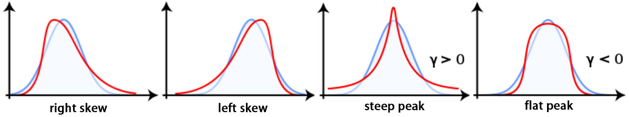
- Skewness: $\tilde{\mu}_ 3=\mathbb{E}[(\mathcal{X}-\mu_ \mathcal{X})^3]/\sigma_\mathcal{X}^3$ ($\tilde{\mu}_ 3>0$ right-skewed, $\tilde{\mu}_ 3<0$ left-skewed)
- Kurtosis: $\tilde{\mu}_ 4=\mathbb{E}[(\mathcal{X}-\mu_ \mathcal{X})^4]/\sigma_\mathcal{X}^4$
- Excessive Kurtosis: $\gamma = \mu_ 4-3$
- Correlation: $\text{corr}(\mathcal{X}_i,\mathcal{X}_j)=\mathbb{E}[\mathcal{X}_i\mathcal{X}_j]$
- Correlation matrix: $C=\mathbb{E}[\mathcal{X}_i\mathcal{X}_j^\top]$
- Correlation coefficient: $\rho(\mathcal{X}_ i,\mathcal{X}_ j)=\frac{\text{corr}(\mathcal{X}_ i,\mathcal{X}_ j)}{\sigma_{\mathcal{X}_ i}^2\sigma_{\mathcal{X}_ j}^2}$
- Covariance: $\text{cov}(\mathcal{X}_i,\mathcal{X}_j)=\mathbb{E}[(\mathcal{X}_i-\mu_i)(\mathcal{X}_j-\mu_j)]$
- Covariance matrix: $S=\mathbb{E}\left[(\mathcal{X}-\mu_ \mathcal{X})(\mathcal{X}-\mu_ \mathcal{X})^\top\right]$
- Properties: $\text{cov}(\mathcal{X}+c)=\text{cov}(\mathcal{X}), \text{cov}(A\mathcal{X},\mathcal{X}B)=A\text{cov}(\mathcal{X})+\text{cov}(\mathcal{X})B^\top$
- Uncorrelated: $\rho(\mathcal{X}_ i,\mathcal{X}_ j)=0 \Leftrightarrow\text{cov}(\mathcal{X}_i,\mathcal{X}_j)=0\Leftrightarrow\text{corr}(\mathcal{X}_i,\mathcal{X}_j)=\mathbb{E}[\mathcal{X}_i]\mathbb{E}[\mathcal{X}_j]$ (uncorrelated is necessary for independent)
- Cases where uncorrelated implies independence: (1) Jointly Gaussian (2) Bernoulli
- Centered variable: $\tilde{\mathcal{X}}=\mathcal{X}-\mu_ \mathcal{X}$
Transform methods
- Probability generating function(PGF): similiar to Z-tranform $$G_ \mathcal{X}(z)\equiv\mathbb{E}[z^\mathcal{X}]=\sum_{x_i}z^{x_i}p_ \mathcal{X}(x_i)$$
- For $\mathcal{F}_ \mathcal{X}=\mathbb{N}$, we have $$\frac{\mathrm{d}^k}{\mathrm{d}z^k}G_ \mathcal{X}(z)\Biggr|_{z=1}=\mathbb{E}[\mathcal{X}(\mathcal{X}-1)\cdots(\mathcal{X}-(k-1))]$$
- Moment generating function(MGF): similar to Laplace transform $$M_ \mathcal{X}(z)\equiv\mathbb{E}[e^{s\mathcal{X}}]=\int^\infty_{-\infty}e^{sx}f_ \mathcal{X}(x)\mathrm{d}x$$
- Generally we have $$\frac{\mathrm{d}^k}{\mathrm{d}s^k}M_ \mathcal{X}(s)\Biggr|_{s=0}=\mathbb{E}[\mathcal{X}^k]$$
- Characteristic function(CF): similar to Fourier transform $$\phi_ \mathcal{X}(\omega)\equiv\mathbb{E}[e^{j\omega \mathcal{X}}]=\int^\infty_{-\infty}e^{j\omega x}f_ \mathcal{X}(x)\mathrm{d}x$$
- Generally we have $$\frac{\mathrm{d}^k}{\mathrm{d}\omega^k}\phi_ \mathcal{X}(\omega)\Biggr|_{\omega=0}=j^k\mathbb{E}[\mathcal{X}^k]$$
- Independent: $\mathcal{X}\perp \!\!\! \perp\mathcal{Y}$ iff. $\phi_ \mathcal{XY}(\omega)=\phi_ \mathcal{X}(\omega)\phi_ \mathcal{Y}(\omega)$
- Joint characteristic function: for vector case $\mathcal{X}\in\mathbb{R}^n$, we define vector $u$ and $$\phi_ \mathcal{X}(u)\equiv\mathbb{E}[e^{ju^\top \mathcal{X}}]$$
- Trivial usage: if $\mathcal{Y}=\mathcal{X}_ 1+\mathcal{X}_ 2$, then $\phi_ \mathcal{Y}(u)=\phi_{\mathcal{X}_ 1}(u)\phi_{\mathcal{X}_ 2}(u)$
Common distributions1
- Bernoulli: $\Omega_\mathcal{X}=\{0,1\}$ $$p_\mathcal{X}(1)=p,\;p_\mathcal{X}(0)=q=1-p$$
- $\mu_\mathcal{X}=p,\;\sigma^2_\mathcal{X}=pq,\;G_\mathcal{X}(z)=q+pz$
- Binomial - $\mathcal{B}(n,p)$: $\Omega_\mathcal{X}=\{0,1,\ldots,n\}$ $$p_\mathcal{X}(k)=\binom{n}{k}p^k(1-p)^{n-k}$$
- $\mu_\mathcal{X}=np,\;\sigma^2_\mathcal{X}=np(1-p),\;G_\mathcal{X}(z)=(1-p+pe^z)^n$
- Multinomial: $\Omega_\mathcal{X}=\{0,1,\ldots,n\}^k$ $$p_\mathcal{X}(x)=\binom{n}{x_1!\cdots x_k!}p_1^{x_1}\cdots p_k^{x_k}$$
- Geometric: $\Omega_\mathcal{X}=\mathbb{N}$ $$p_\mathcal{X}(k)=(1-p)^{k-1}p$$
- $\mu_\mathcal{X}=\frac{1}{p},\;\sigma^2_\mathcal{X}=\frac{1-p}{p^2},\;G_\mathcal{X}(z)=\frac{pz}{1-(1-p)z}$
- Poisson: $\Omega_\mathcal{X}=\mathbb{N}$ $$p_\mathcal{X}(k)=\frac{\lambda^k}{k!}\exp\{-\lambda\}$$
- $\mu_\mathcal{X}=\lambda,\;\sigma^2_\mathcal{X}=\lambda,\;G_\mathcal{X}(z)=\exp\{\lambda(z-1)\}$
- Uniform - $\mathcal{U}(a,b)$: $\Omega_\mathcal{X}=[a,b]$ $$f(x)=
\begin{cases}
1/(b-a)&,\;x \in [a,b] \\
0&,\;\text{otherwise}
\end{cases}$$
- $\mu_\mathcal{X}=\frac{1}{2}(a+b),\;\sigma^2_\mathcal{X}=\frac{1}{12}(b-a)^2,\;M_\mathcal{X}(s)=\frac{e^{sb}-e^{sa}}{s(b-a)}\;(s\neq 0)$
- Normal - $\mathcal{N}(\mu,\sigma)$: $\Omega_\mathcal{X}=\mathbb{R}$
$$f(x)=\frac{1}{\sqrt{2\pi\sigma}}\exp\left\{-\frac{(x-\mu)^2}{2\sigma^2}\right\}$$
- $M_\mathcal{X}(s)=\exp\left\{\mu s+\frac{1}{2}\sigma^2s^2\right\}$
- Joint Normal: $\Omega_\mathcal{X}=\mathbb{R}^n$
$$f(x)=\frac{1}{\sqrt{(2\pi)^n \det(S)}}\exp\left\{-\frac{1}{2}(x-\mu)^\top S^{-1}(x-\mu)\right\}$$
- $\phi_\mathcal{X}(u)=\exp\left\{ju^\top \mu-\frac{1}{2}u^\top Su\right\}$
- Rayleigh: $\Omega_\mathcal{X}=[0,\infty]$ $$f(x)=\frac{x}{\sigma^2}\exp\left\{-\frac{x^2}{2\sigma^2}\right\}H(x)$$ where $H(x)$ is Heaviside step function
- Exponential - $\mathcal{E}(\lambda)$: $\Omega_\mathcal{X}=[0,\infty]$ $$f(x)=\frac{1}{\mu}\exp\left\{-\frac{x}{\mu}\right\}H(x)$$
- $\mu_\mathcal{X}=1/\lambda,\;\sigma^2_\mathcal{X}=1/\lambda^2,\;M_\mathcal{X}(s)=\lambda/(\lambda-s)$
- Laplacian: $$f(x)=\frac{1}{2b}\exp\left\{-\frac{|x-\mu|}{b}\right\}$$
Derivation of the distributions
- Bernoulli → Binomial: $\mathcal{X}_ i\sim\text{Bernoulli}( p) \Rightarrow \mathcal{Y}=\sum_{i=1}^n \mathcal{X}_ i\sim\mathcal{B}(n,p)$
- Bernoulli → Geometric: $\mathcal{X}_i\sim\text{Bernoulli}( p) \Rightarrow \mathcal{Y}\sim\text{Geometric}( p)$ denoting the first $\mathcal{X}_i=1$
- Binomial → Poisson: $\mathcal{X}_i\sim\mathcal{B}(n,p,k=1) \Rightarrow \mathcal{Y}\sim\text{Poisson}(\lambda)$ when $n\to \infty$ with $p=\frac{\lambda\tau}{n}$
- Binomial → Exponential: $\mathcal{X}_i\sim\mathcal{B}(n,p,k\neq0) \Rightarrow \mathcal{Y}\sim\mathcal{E}(\lambda)$ when $n\to \infty$ with $p=\frac{\lambda\tau}{n}$
Actually $\mathcal{B}(n,p,k) \Rightarrow e^{-\lambda \tau}\frac{(\lambda \tau)^k}{k!}$
- Exponential → Laplacian: $\mathcal{X}_1, \mathcal{X}_2 \sim\mathcal{E}(\lambda) \Rightarrow \mathcal{X}_1-\mathcal{X}_2\sim\text{Laplacian}(\lambda^{-1})$
Concentration Inequalities
- Cauchy-Schwarz Inequality: $S=\left(\mathbb{E}[\mathcal{X}\mathcal{X}_j]\right)^2\leqslant\left(\mathbb{E}[\mathcal{X}_i]\right)^2\left(\mathbb{E}[\mathcal{X}_j]\right)^2$
- Markov Inequality: $\mathbb{P}(\mathcal{X}\geqslant a)\leqslant \mathbb{E}\mathcal{X}/a,\;a>0$
- Chebychev Inequality: $\mathbb{P}(|\mathcal{X}-\mu|\geqslant\delta)\leqslant\sigma^2/\delta^2$
- Jenson Inequality: $\psi(\mathbb{E} \mathcal{X}) \leqslant \mathbb{E}\psi(\mathcal{X})$ for any convex function $\psi$
- Chernoff bound: $\mathbb{P}(\mathcal{X}\geqslant a)\leqslant \underset{s\geqslant 0}{\min},e^{-as}M_ \mathcal{X}(s)$
- Law of Large Numbers: let $\mathcal{X}_i$ be samples drawn from $(\mathbb{R}^n,\mathcal{F}^n,\mathbb{P})$, and $\mathbb{P}$ is such that $\mathcal{X}_k$ has mean $\mu$ and covariance $S$
- Weak version: if $\mathcal{Y}_ k=\frac{1}{k}\sum^k_{j=1}\mathcal{X}_j$ then $$\underset{k\to\infty}{\lim} \mathbb{P}\left(\left\Vert \mathcal{Y}_k-\mu\right\Vert>\epsilon\right)=0$$
- Strong version: if $\mathcal{Y}_ k=\frac{1}{k}\sum^k_{j=1}\mathcal{X}_j$ then $$\underset{k\to\infty}{\lim} \mathcal{Y}_k=\mu$$
- Central Limit Theorem: if $\mathcal{Y}_ k=\frac{1}{\sqrt{k}}\sum^k_{j=1}S^{-1/2}\left(\mathcal{X}_ j-\mu\right)$ then $$\underset{k\to\infty}{\lim} f_{\mathcal{Y}_k}(y_k)=\mathcal{N}(0,I)$$
Estimation Theory
- Hilbert Space Projection Theorem: A Hilbert space is a complete inner product space. Let $\mathcal{H}$ be a Hilbert space, $\mathcal{M}$ be a closed subspace of $\mathcal{H}$ and $z\in\mathcal{H}$. Then there is a unique $\hat{z}\in\mathcal{M}$ which is closest to $z$: $$\Vert z-\hat{z}\Vert < \Vert z-y\Vert, \forall y\in\mathcal{M}, y\neq\hat{z}$$
- Orthogonality Principle: $\hat{z}$ is the closest point iff. $\langle z-\hat{z},y\rangle=0, \forall y\in\mathcal{M}$. In estimation we formulate inner product as $\langle \mathcal{X}, \mathcal{Y}\rangle=\mathbb{E}[\mathcal{X}\mathcal{Y}^T]$, it’s $\mathbb{E}[(\mathcal{Y}-\mathbb{E}[\mathcal{Y}|\mathcal{X}])h(\mathcal{X})]=0, \forall h(\cdot)$.
- Estimation Problem: Given random vector \mathcal{X} and random variable $\mathcal{Y}$ with joint PDF $f_{\mathcal{XY}}(\cdot)$, we observe $\mathcal{X}=x$ and we want to form an estimate of $\mathcal{Y}$ as $\hat{\mathcal{Y}}=g(x)$
- Minimum Mean Square Error(MMSE) Estimation: $\hat{\mathcal{Y}}=\mathbb{E}(\mathcal{Y}|\mathcal{X})$
- Target: minimize $\mathbb{E}[(\mathcal{Y}-\hat{\mathcal{Y}})(\mathcal{Y}-\hat{\mathcal{Y}})^\top]$ with $\hat{\mathcal{Y}}=g(\mathcal{X})$ (arbitary $g(\cdot)$)
- Linear Minimum MSE(LMMSE) Estimation: $\hat{A}$ satisfies $\mathbb{E}[\mathcal{YX^\top}]=A\mathbb{E}[\mathcal{XX^\top}]$
- Target: minimize $\mathbb{E}[(\mathcal{Y}-\hat{\mathcal{Y}})(\mathcal{Y}-\hat{\mathcal{Y}})^\top]$ with $\hat{\mathcal{Y}}=A\mathcal{X}$
- Affine Minimum MSE(AMMSE) Estimation: $\hat{G}$ satisfies $\mathbb{E}[\mathcal{YX^\top}]=G\mathbb{E}[\mathcal{XX^\top}]$, $\hat{c}=\mu_{\mathcal{Y}}-\hat{G}\mu_{\mathcal{X}}$
- Target: minimize $\mathbb{E}[(\mathcal{Y}-\hat{\mathcal{Y}})(\mathcal{Y}-\hat{\mathcal{Y}})^\top]$ with $\hat{\mathcal{Y}}=G\mathcal{X}+c$
Convergence
- Categories: Generally we assume $n\to\infty$ and giving $\mathcal{X}_n$ are random variables.
- Sure Convergence ($\mathcal{X}_n\xrightarrow{\text{surely}}\mathcal{X}$): $$\forall \omega\in\Omega, \mathcal{X}_n(\omega)\xrightarrow{n\to\infty}\mathcal{X}$$
- Almost Sure Convergence ($\mathcal{X}_ n\xrightarrow{\text{a.s./w.p.1}}\mathcal{X}$,
w.p.1: with probability 1): $$\mathbb{P}(\{\omega\in\Omega:\lim_ {n\to\infty}\mathcal{X} _n(\omega)=\mathcal{X}\})=1$$- Equivalent definition: $$\mathbb{P}(\bigcup_{\epsilon>0}A(\epsilon))=0\;\text{where}\;A(\epsilon)=\bigcap_{N=1}\bigcup_{n=N}\{\omega:|\mathcal{X}_n(\omega)-\mathcal{X}(\omega)|\geqslant\epsilon\}$$
- Convergence in Probability ($\mathcal{X}_ n\xrightarrow{\text{in prob.}}\mathcal{X}$): $$\mathbb{P}(\{\omega\in\Omega:\lim_ {nn\to\infty}|\mathcal{X}_n(\omega)-\mathcal{X}(\omega)|\geqslant\epsilon\})=0,\;\forall\epsilon>0$$
- Convergence in Distribution ($\mathcal{X}_ n\xrightarrow{\text{D}}\mathcal{X}$): $$\lim_ {n\to\infty} F_{\mathcal{X}_ n}(x)=F_{\mathcal{X}}(x)$$
- Convergence in mean of order: ($\mathcal{X}_ n\xrightarrow{\text{mean r}}\mathcal{X}$, abbr.
m.s.for $r=2$): $$\mathbb{E}[|\mathcal{X}_n-\mathcal{X}|^r]\to 0$$ - $\mathcal{X}_n\xrightarrow{\text{a.s./mean r}}\mathcal{X}\Rightarrow\mathcal{X}_n\xrightarrow{\text{in prob.}}\mathcal{X}\Rightarrow\mathcal{X}_n\xrightarrow{\text{D}}\mathcal{X}$
- Strong Law of Large Numbers (requires iid.): $$S_n=\frac{1}{n}\sum\mathcal{X}_ i\xrightarrow{\text{a.s./m.s.}}\mu_ \mathcal{X}$$
- Weak Law of Large Numbers (requires indentical uncorrelated distributed): $S_n\xrightarrow{\text{in prob.}}\mu_\mathcal{X}$
- Central Limit Theorem (requires independent): $$\mathcal{Y}_n=\frac{1}{\sqrt{n}}\sum\frac{\mathcal{X}_i-m}{\sigma}\xrightarrow{\text{D}}\mathcal{N}(0,1)$$
Law of Large Numbers and Central Limit Theorem together characterized the limiting behavior of the average of samples. See Wikipedia and a proof to see their relationships.
Miscellaneous Corollaries
- For random valuable that takes positive values, $\mathbb{E}(X)=\int^\infty_0 \mathbb(\mathcal{X}>x)dx$
- If $\mathcal{X}_1,…\mathcal{X}_n$ are IID continuous random variables, then $\mathbb{P}(\mathcal{X}_1<\mathcal{X}_2<\ldots<\mathcal{X}_n)=1/n!$
- Define $\mathcal{X}_ {(j)}$ to be the j-th smallest among $\mathcal{X}_ 1,…\mathcal{X}_ n$. Suppose $\mathcal{X}_ 1,…\mathcal{X}_ n$ are IID random variables with PDF $f$ and CDF $F$, then $$f_ {\mathcal{X}_ {(j)}}(x)=\frac{n!}{(n-j)!(j-1)!}[F(x)]^{j-1}[1-F(x)]^{n-j}f_ \mathcal{X}(x)$$